

Most excel users confuse cell gridlines and cell borders. Excel gridlines are customized differently to the borderline. In excel, gridlines are displayed using a default color assigned by excel. If you need to change the color of the gridline for your worksheet, it's possible. To most users, you know hiding gridlines is common. In some cases, gridlines are beneficial, but, in some cases, hiding gridlines are needed. It is important to know that gridline makes data more readable without borders.
We have a different method to hide the gridline.
Method 1
Use of option in the ribbon
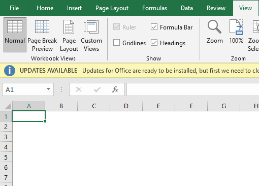
1. Every version of excel has a default function to hide mesh lines. Go to the "view tab" on the excel ribbon.

2. In the view tab, you will see a check box named gridline. Uncheck the box. And all the mesh will be hidden.

3. It's a default function. The output will be like this.
Method 2
Hide gridlines by changing the background color.
It is quite an obvious method of hiding the gridline.
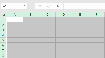
Select all rows and columns in any way or click CTRL + A. Another way is to click the triangle icon under the name box.
1. Select everything in the worksheet.
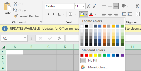
2. Click fill, color option, and select the color your option.
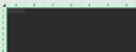
3. After selecting the color option, all the gridlines will disappear. The output will be like this.
If you want all cells, you can hover the cursor over the worksheet. All cells will be displayed as the mouse moves around.
Keyboard shortcut.
4. We love to be seen as pros. Keyboard shortcut makes work easy and fast. ALT+WVG key combination will hide excel grid bars. Sometimes all borders and gridlines will disappear. As shown in the screenshot below
Hide gridline for specific cells
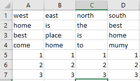
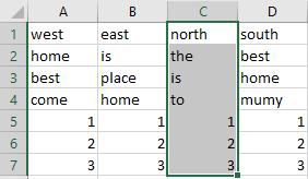
In most cases, we need to hide a specific block of cells. We can use the white cell background or apply the white border. Let's remove the gridline by coloring the border. Let's use this example.
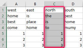
1. Select the range of cells you want to remove the gridlines.
2. Right-click on the selection. Choose format cells.
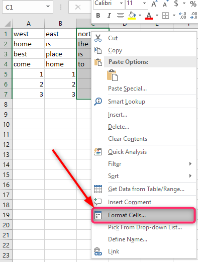
You can use CTRL + 1 to get the format cell.
3. While in the format cell, selects the border tab.
In the color section, chooses white color. In the preset region, click inside and outline.

4. Click ok to see the changes.
Change the color of gridlines. As you can see, all the gridlines have gone. You can select the whole table and change the color to white if you want. This will be easy and fast. You can use other options like using the VBA script and printing the worksheet. I prefer to change the color of gridlines as it won't consume a lot of time. Other tricks are complex; the complex procedures are fast and work with large data content or many worksheets. Try to learn many of these tricks if you are a frequent user of excel.