
Sometimes you may get data attached to some other data that you don't require. Luckily, Excel allows you to get rid of the extra characters. In this tutorial, we are going to look at how you can eliminate the last 4 characters.
Apart from removing the last characters, you can also remove the first characters that you do not need. That is the characters on your left or right. The best thing about all this is that you can remove these characters using a simple formula/ function or using software known as KUTOOLs.
Using the left function
If you are removing the last characters the left function is the most appropriate to use. Conversely, you can use the right Function to remove the first characters from the beginning of a text string.
Steps
1. Open your spreadsheet
2. Enter the following formula in an empty cell =LEFT(A1, LEN(A1)-4)
3. Press enter and the characters will be removed

4. Right Click and drag the green rectangle to the rest of the cells

In the example above we have removed the last four characters. This formula can be used to remove as many characters as you want. Just replace 4 with the number of characters that you want to eliminate.
Using VBA code for a user-defined function
Another easy way that you can remove both the first and last characters is by using the user-defined function.
Steps
1. Press Alt+F11 to open the window for Microsoft Visual Basic

2. Click insert module

3. Copy and paste the code below to the script editor
Sub Remove_Last_Character()
On Error GoTo Message
Dim n As Integer
n = Int(InputBox("Enter the Number of Last Characters to Remove: "))
For i = 1 To Selection.Rows.Count
For j = 1 To Selection.Columns.Count
Selection.Cells(i, j) = Left(Selection.Cells(i, j), Len(Selection.Cells(i, j)) - n)
Next j
Next i
Exit Sub
Message:
MsgBox "Please Enter a Valid Integer Less than or Equal to the Length of the Strings."
End Sub
4. save the code and return it to your spreadsheet
5. Highlight your data Press ALT+F8

6. Select the Remove_Last_Character Macro and click run

7. Enter 4 as the number of characters you wish to remove and click okay.

8. All the last four columns will be removed

The above two methods are very easy and they work with all versions of excel.
Use KUTOOLS software to remove the last 4 characters
Download KUTOOLS File from here and install it on your computer. This is will appear as a tab on your Excel and you can use it to simplify so many processes and manage your documents painlessly. Besides, it is a very small file of 48 MBS. Installation is easy and it does not upload any data or obtain any useful information.
Steps for removing the last 4 characters using KUTOOLS
1. Download and install KUTOOLS

2. Restart your Excel app
3. Click on Kutools >>Text and select remove by position

4. Enter the number of characters that you want to remove in the pop-up box that will appear.

5. Select the position that you want, i.e. right or left, and click apply.
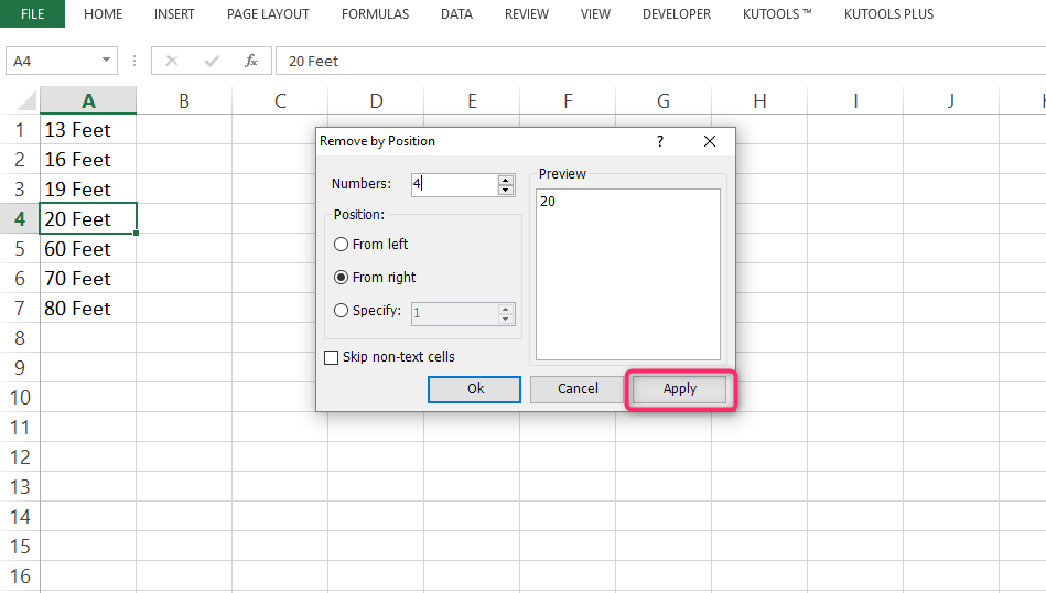
6. The last four digits will be removed

You can also select as many cells as you can and eliminate the characters using kutools. Keep it as you are going to use it a lot as you work with Excel. I highly recommend using kutools as it is easy to install and use.
Using the REPLACE Function
The REPLACE Function can easily remove the last characters from a number, and its formula is =VALUE(REPLACE(B5,LEN(B5),N," ")), where;
B5 is the old text
LEN(B5) returns the length of the old text.
N is the number of characters you want to remove.
" " is the new text (blank)
The formula will convert the string into a new text or number. You can easily remove the last 4 characters through these simple steps:
We’ll use data in the following image in our illustrations below;

1. Type =REPLACE(D5; FIND(" ";D5)+1; 4; "") in cell K5.

2. Press Enter button and you have the output.
3. Use the Fill Handle icon to drag the formula down to other cells.

Using the MID Function
The MID function can remove any number of last characters from your old text. Its formula is =MID(DN,1,LEN(DN)-N), where:
DN is the old text and N represents the number of characters in the original text.
1 is the start number.
LEN(DN)-N is the number of characters you want to remove. In this case, it will be LEN(DN)-4.
Steps:
1. Write the formula in cell E5. For example, =MID(J5,1,LEN(J5)-4).

2. Press Enter button and you will the output in the cell

3. Use the Fill Handle icon to drag the formula down to other cells.
4. The resulting text will show in the corresponding cells with the last four characters omitted.

Using Flash Fill Technique
You can also remove the last four characters using the Flash Fill function in Excel. In this case, you need to create a new column to store the new text once the last four characters are removed from the old text. To use this formula, follow these steps:
1. Create a column by selecting cell K5.
2. Type the new title you want to appear in cell K5.

3. The method allows you to remove the characters manually.
4. In other cells below K5, start typing the previous text and the new text will be suggested.

5. Press Enter and the new texts will appear with the last four digits removed.
Using VBA Code
The VBA Code is another user-defined function that allows you to remove the last characters from a text easily. It works similarly to the LEFT and REPLACE functions, though in this case, you have to use Developer options already available in Excel. You can also get the VBA code by pressing the Alt+11 keys. When using Developer options, follow these steps:
1. Click on the Developer tab in Excel and select Visual Basic

2. When Visual Basic Editor opens, select the Insert Tab and open the Module

3. This will create Module 1. Write this code in the module:
Public Function RmvLstCh(txt As String, char_no As Long)
RmvLstCh = Left(txt, Len(txt) - char_no)
End Function

4. Writing the code will create an RmvLstCh function. Save the code and close the window.

5. Back to your old text, create another column to store the new text
6. Type the =RemoveLast4Characters(J5;4) formula in cell K5, where J5 is the old text, and 4 is the number of characters to remove.

7. Press Enter and you will see the output in the formula cell.

8. Drag the formula down using the Fill Handle icon to other cells in the column.
9. You will finally see the new text with the last four characters removed.