There are various methods of returning a value from a Table array based on more than one criteria. Vlookup is used when there is only one criterion (condition). In this tutorial, we will be discussing the method involving INDEX and MATCH.
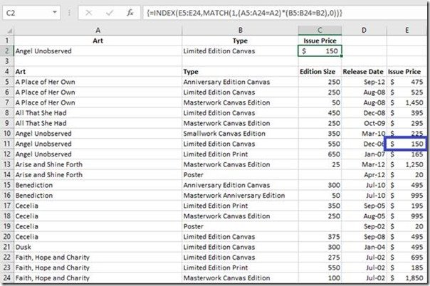
Let us consider an example, see the below illustration:

The Formula in C2 is:
{= INDEX (E5:E24, MATCH (1, (A5:A24=A2) * (B5:B24=B2), 0))}
The above formula is an array formula so for it to work, instead of using the Enter key, you must use CONTROL + SHIFT + ENTER
Here is how the formula works
In the above example, we are looking up the Issue Price of an item with the Art Name of “Angel Unobserved” and Type “Limited Edition Canvas”. The first Excel Function that comes to mind is VLOOKUP but in this instance, VLOOKUP will not give the accurate Issue Price because we have more than one occurrence of “Angel Unobserved” plus VLOOKUP only works when one condition is to be met. VLOOKUP would return the Issue Price of the first “Angel Unobserved” it finds.
MATCH returns the location of an item in an array.
=MATCH (1, (A5:A24=A2) * (B5:B24=B2), 0
Here, we asked the MATCH function to search for 1 in an array we built from scratch. This array, A5:A24=A2, looks for A2 in A5:A24 and returns an array of TRUEs (which means 1 mathematically) and FALSEs (which is 0 mathematically).
{FALSE; FALSE; FALSE; FALSE; FALSE; TRUE; TRUE; TRUE; FALSE; FALSE; FALSE; FALSE; FALSE; FALSE; FALSE; FALSE; FALSE; FALSE; FALSE; FALSE}
TRUE for when it finds a match and FALSE for no match. The same thing goes for (B5:B24=B2).
{FALSE; TRUE; FALSE; TRUE; FALSE; FALSE; TRUE; FALSE; FALSE; FALSE; FALSE; FALSE; FALSE; FALSE; FALSE; TRUE; TRUE; TRUE; FALSE; FALSE}
Multiplying the 2 arrays will give an array of 1 and 0’s because 1×1=1, 1×0=0, and 0x1=0. So, MATCH will then return the location of the only 1 in the array, which is 7
{0; 0; 0; 0; 0; 0; 1; 0; 0; 0; 0; 0; 0; 0; 0; 0; 0; 0; 0; 0}
The last bit of this netted formula is the INDEX function. INDEX returns the value at the intersection of a row and column in a range. So, in the specified array, E5:E24, MATCH gives the position of what we are looking for, which is the 7th cell in the E4:E24 array.
=INDEX (E5:E24, 7)
Remember to make use of CONTROL + SHIFT + ENTER because this is an array formula.

