

A correlation coefficient shows the relationship between two variables; the value should lie between -1 and 1. It simply shows how much an independent variable explains a dependent variable. Fortunately, you can now quickly calculate correlation co-efficient on an Excel worksheet using the following methods.
Method 1: Use the CORREL Function
Assume you have two sets of data; one is the A variable, and the other is the B variable. If you were to find their correlation coefficient:
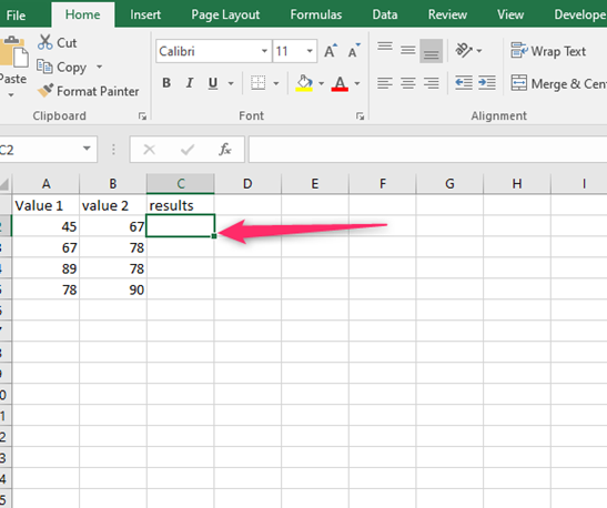
1. Select a Blank Cell
You will put your calculation result on the selected blank cell.
2. Fill the formula =CORREL(A2:A7, B2:B7)
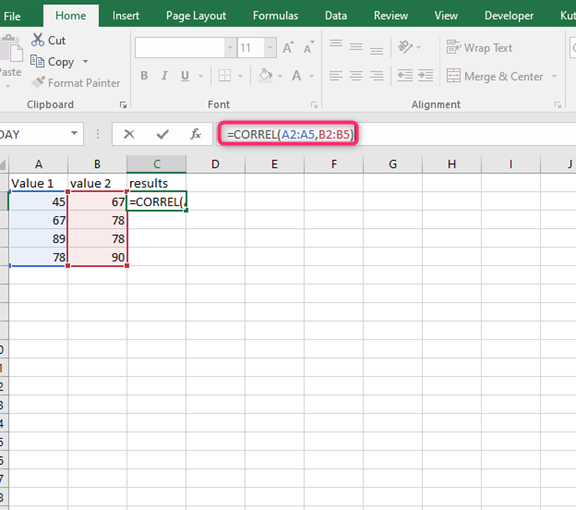
The formula can also be written as =CORREL (array1, array2)
That is;
- 'array1' – required cell range (can be X)
- 'array2' – required cell range (can be Y)
This formula compares two sets of variables and can also be applied to any other range of cells.
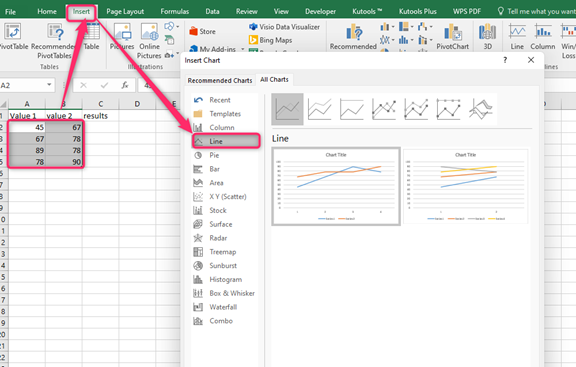
3. Optionally, insert a line chart.
The line chart will enable you to see the relationships between the two coefficients. For instance, you will see a red line representing the A variable and a blue line representing the B variable.
4. Press "Enter" to find the correlation coefficient.
As long as you replace the formula with the correct cell references, you will always find an accurate answer in Excel.
Method 2: Applying Data Analysis and Outputting the Analysis
The Analysis Toolpak calculates the correlation coefficient of more than two data sets. To calculate the correlation coefficient using the Analysis Toolpak add-in in Excel:
1. Find the Data Analysis add-in
First, confirm that your device has the Data Analysis add-in on the Data group.
2. Click "Files" in Excel
3. Click "Options"
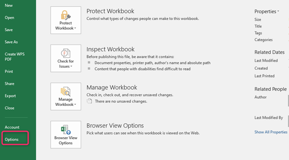
An Excel Options window will pop. On the left side of the window, click on "Add-ins," then click "Go" on the drop-down list. An add-ins dialogue box will open.

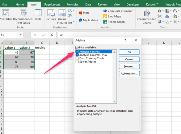
4. Select "Analysis Toolpak."
Click "OK" to add the add-in on your worksheet's tab; the analysis toolpak provides data analysis and statistics tools.
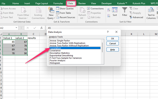
5. Next, click "Data."
You will find the icon on the data analysis dialog. Then, pick correlation and select 'OK" The correlation dialog will open. On the correlation dialog box;
- Add the data range; it is the range of cells between your X and Y variables.
- Use your data to select columns and rows.
- If your data has any labels, select "Labels in the first row."
- Select the option suitable for your data in the outputs option, whether the output range, new worksheet ply, or the new workbook. The output range is the cell where you want the result to appear.
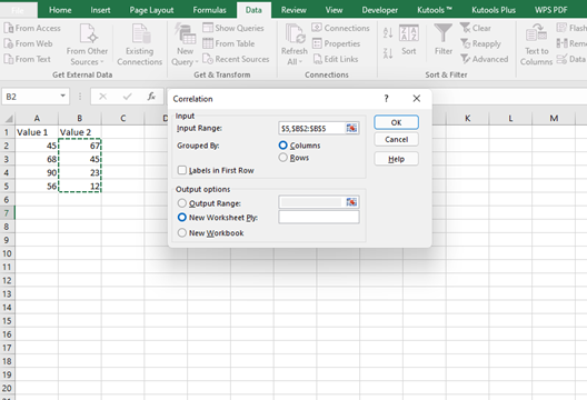
6. Lastly, click "OK."
You will see the result of the correlation coefficient of your variables on your Excel worksheet.
Note
If you find a correlation coefficient of 0, there is no relationship between any variables in question.
If you find a correlation coefficient of -1, your variables have a strong negative relationship.
If you find a correlation coefficient of +1, your variables have a strong positive relationship.