

The comparison involves checking if one list matches the other. Excel is a powerful tool for checking if one column matches the data in the other column. This is because excel consists of cells that are arranged in columns. Therefore, few workarounds and formulas can be used to check the comparison between two or more columns. In this article, we shall discuss some of the common ways to compare columns in excel.
Comparing Columns Using CountIf formula
COUNTIF is an in-built formula used in Excel to execute various operations in Excel. In comparing columns data, the Countif formula has proved to be mighty. Let us discuss some of the steps followed when using this method:
1. Enter the data to be compared, or open the existing that you want to check the difference.
2. Ensure your data is in two or more columns.

3. Then, create a separate column that will contain the feedback of the comparison.
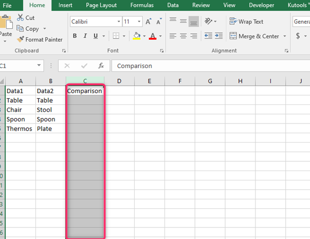
4. On the feedback column, click on the first blank cell and enter this formula.
=IF(COUNTIF($B:$B, $A2)=0, "No match found")
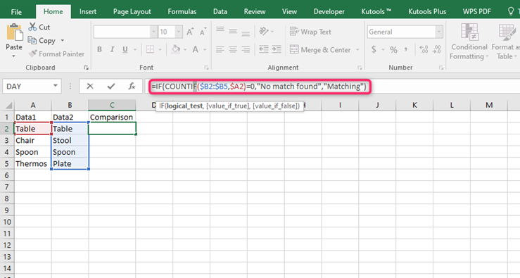
The formula returns zero if no match is found. Therefore, it can check the difference of the data contained in the column in question.
5. Drag the formula to other cells and check the difference between the columns.
Comparing two columns using rows
Another way to check the differences in the column is by using row data. While using this technique, the IF function is used. The data of column 1 is compared to that of column 2. That is IF(column1=column2) return true.
Steps:
1. Enter the data to be compared, or open the existing that you want to check the difference.
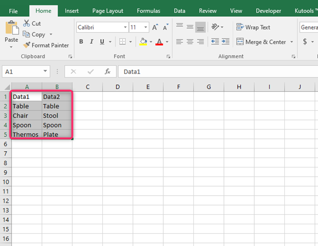
2. Ensure your data is in two or more columns. Create a separate column where you will input the formula.
3. Enter the IF function to compare the two rows in the third column.
=IF (A2=B2, "match," "no match")
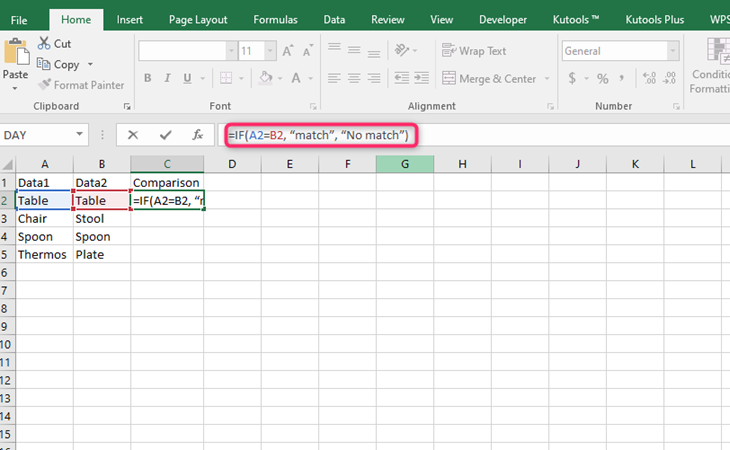
If the formula returns a match, there's no difference in the data found in column 1 and that found in column 2.
On the other side, if the IF function returns No match, there's a difference between the data in column 1 and column 2.
Comparing using conditional formatting feature
A conditional formatting tool compares the data and highlights. It can be used to show the difference in two-column or more. Here are the steps followed when using this feature:
1. Enter the data to be compared, or open the existing that you want to check the difference.
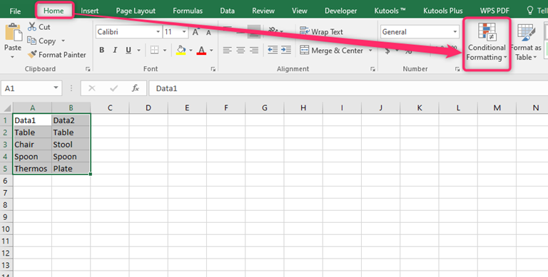
2. Highlight the two-column that contain your data.
3. On the Home tab, click the Conditional formatting button.
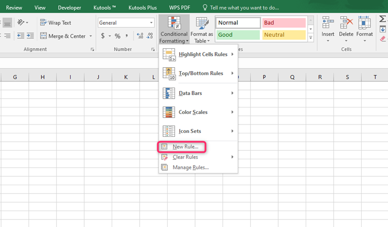
4. From the drop-down menu, select the new rule button.
5. On the Edit formatting rule dialogue box, click the use a formula to determine which cells to format. Type the comparison formula on the formula bar.
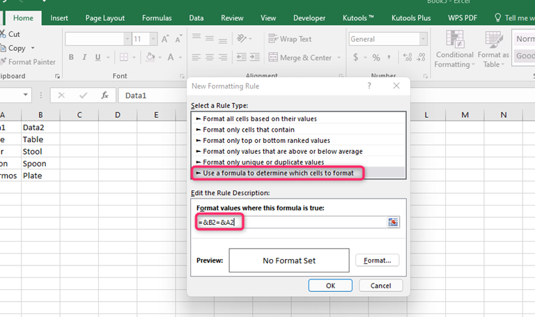
6. Finally, format the color that will differentiate between the cells that match the formula.
