

The conditional Formatting Tool is used to perform various functions in Excel. One of the most significant tasks performed by conditional formatting is highlighting cells with the matching rule. However, did you know you can use this tool to check dates? Excel uses manual methods in most cases to highlight dates and count days older than the specified date. The manual methods prove to be tedious and time-consuming. Hence there is a need to automate the process.
To Highlight Dates older than two weeks
Here are the steps to follow:
1. Open the Excel application.
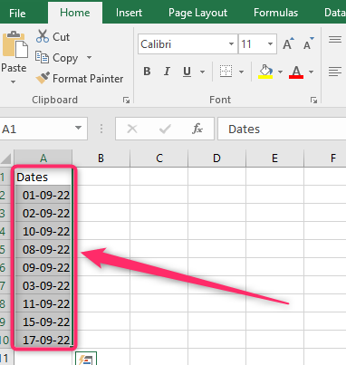
2. Open the Workbook containing the dates you wish to check if they are older than two weeks. Select all the cells with the dates you wish to check.
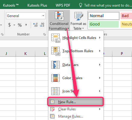
3. Click the Home tab on the Ribbon, and locate the Styles section. Under this section, click the Conditional Formatting drop-down button.

4. Choose the New Rule button from the menu to open the Edit Formatting Rule dialogue box.
5. In the Edit Formatting Rule dialogue box, choose the “Use a Formula to determine which cells to format” option in the “Select a Rule Type” section.
6. In the Edit Rule Description section, type this formula =A2<TODAY()-14

Note: There are 14 days in two weeks.
The A2 in the formula indicates the first cell with your dataset in the selected sheet.
7. Click the Format button to open the Format Cells dialogue box. In the dialogue box, click the Fill tab.

8. Next, select the color you wish to highlight the dates. Finally, click the OK button.

To Highlight Dates older than 30 days
Here are the steps to follow:
1. Open the Excel application.
2. Open the Workbook containing the dates you wish to check if they are older than 30 days. Select all the cells with the dates you wish to check.

3. Click the Home tab on the Ribbon, and locate the Styles section. Under this section, click the Conditional Formatting drop-down button.
4. Choose the New Rule button from the menu to open the Edit Formatting Rule dialogue box.
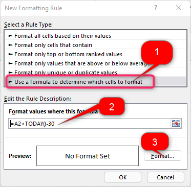
5. In the Edit Formatting Rule dialogue box, choose the “Use a Formula to determine which cells to format” option in the “Select a Rule Type” section.
6. In the Edit Rule Description section, type this formula =A2<TODAY()-30
Note:
The A2 in the formula indicates the first cell with your dataset in the selected sheet.
7. Click the Format button to open the Format Cells dialogue box. In the dialogue box, click the Fill tab.
8. Next, select the color you wish to highlight the dates. Finally, click the OK button.
