Cell reference refers to a unique address. This allows you to reference this cell elsewhere in excel. Cross-referencing is done in the same worksheet, in different worksheets in the same file, and across different workbooks entirely.
A cell is named using a column that uses letters and a row that entails numbers. Cells in different spreadsheets in an Excel workbook will have identical cell references if they occupy the same position in different sheets.
How to cross-reference data between spreadsheets
To cross-reference between spreadsheets, you must identify cells using extended addresses. The extended references identify the cell's sheet, as well as its column and row, follow the steps below.
1. Identify the row you want to reference. For our example, our row is number 2

2. Identify the column that you want to cross-reference and this forms a cell. For our example the column is D.

4. Combine these characters to form a cell address that you want to cross-reference. Example above D2
5. Identify the name of the sheet that you have on your cell. If not named excel gives it a random name as sheet1
6. Combine the cell's address to its sheet's name, separated by an exclamation mark. Example=sheet1!d2 ( is referenced in sheet3.)
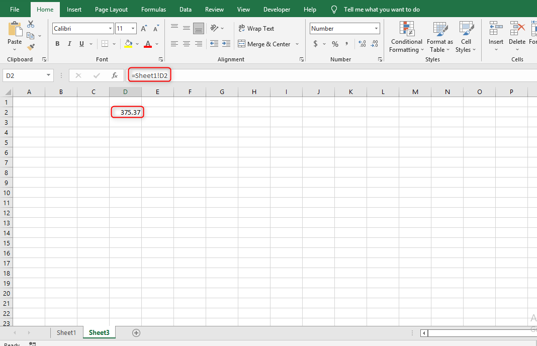
7. Use the extended reference to identify the cell in the formula. Start with an equal sign when writing the formulae.

How to reference from another Excel workbook file
When you link a cell in Excel to another worksheet, the cell that contains the link shows the same info as the cell from the other worksheet that you want to reference. The important thing is to ensure the formula is correct to avoid errors. Follow the below steps to reference another workbook file.
1. Ensure you have both the excel workbooks opened.
2. Type an equal sign (=), switch to the other file, and then click the cell in that file you want to reference and press enter.
3. Identify the workbook name, sheet name, and cell number. In this example, our previous workbook name is a financial sample, the sheet name is sheet1 and the cell is F2.
4. Write them as follows in the formula bar of the workbook you want to refer to. =[FinancialSample.xlsx]Sheet1!D2
5. If the file or sheet name contains spaces, then you will need to enclose the file reference in single quotation marks.= '[Financial Sample.xlsx]Sheet1'!D2

6. When you click enter after the formulae, the results will pop out. Paths to where the document is might come and there is no problem with that.
Referencing both the same workbook and different workbooks helps in the easy management of data. It is also easier to work from a different worksheet or workbook without altering the initial data. The most essential thing is to ensure the formula is correct and the referencing will be automatically correct.
Cross-Reference Your Spreadsheet With VLOOKUP
Imagine you have two lists, they have one column in common names. The first list contains the names of students enrolled, while the second list contains the names of those students who are present.
Steps;
1. Add a new column for the cross-referenced data. Here's how;
In the first new row, enter the VLOOKUP function. Lookup Value element you add the value in this list that you want to use to cross-reference to the other list.
In the Table Tray element, you add the table you want to look up i.e., students present (add the dollar sign to help with copying down the column later)
In the Col Index Num, enter the number of the column in the array you want as the answer, The name of the student is in the 2nd column, so enter 2.
In the Range Lookup always enter False
=VLOOKUP(B4,$B$3:$C$16,2,FALSE)

2. Copy down the column or click and drag down.

Because we put the dollar sign in the Table Array in the first row, we can copy down the column or click-n-drag using the handle.
Now all the values are cross-referenced.
Cross-Reference Excel Spreadsheet Data Using Index/Match
The Index Match formula is a combination of two functions in excel. The Index function returns the values of a cell in a table on the column and row number. While the Match function returns the position of a cell in a row or column.
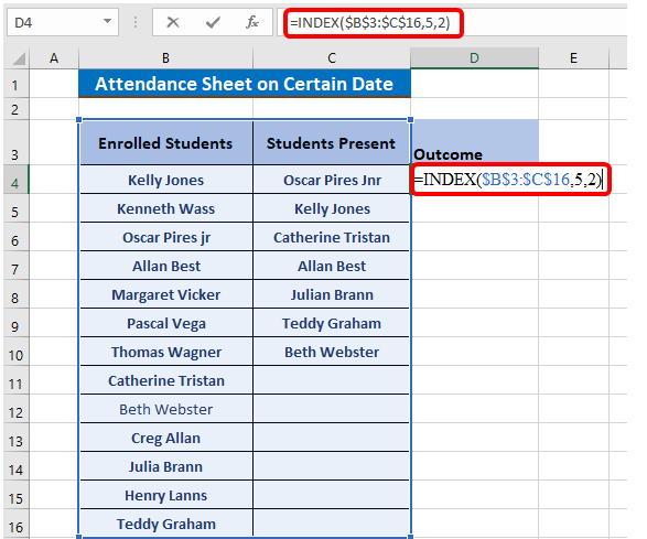
Consider the table showing the names of students enrolled and a list of those present. We want to use the INDEX formula to cross-reference the list

Steps;
Type ‘=INDEX(‘and select the area of the table then add a comma (,)
Type the row number and then comma (,)
Type the column number and close the bracket.
=INDEX($B$3:$C$16,5,2)
Steps;
Using MATCH Formula
1. Type ‘=MATCH(‘and click on the cell containing the name we want to look up
2. Select all the cells in the Name column including the ‘Name’ header
3. Type zero ’0’, then close the bracket
=MATCH(D4,B3:C16,0)

Steps;
1. Type ‘=MATCH(‘and link the cell containing the criteria we want to look up
2. Select all the cells across the top row of the table
3. Type zero ‘0’ for an exact match, then close the bracket
