
In mathematics and other related fields, you may be required to calculate the slope of a given graph. The slope is the steepness of a graph or a given section within the graph. The slope of a graph is used to determine the steepness and the direction of the graph. In math, the slope is denoted using the letter m. The slope of the line can be determined using a formula or chart. This article shall discuss how to determine the slope using the two techniques.
Method 1: Finding slope using a Formula
When calculating the slope of a line, the slope function proves to be the easiest method. The slope function is an in-built function that returns the slope of the line when used. The function only requires two parameters: X and Y values.
=SLOPE (Y values, Xvalues)
Steps:
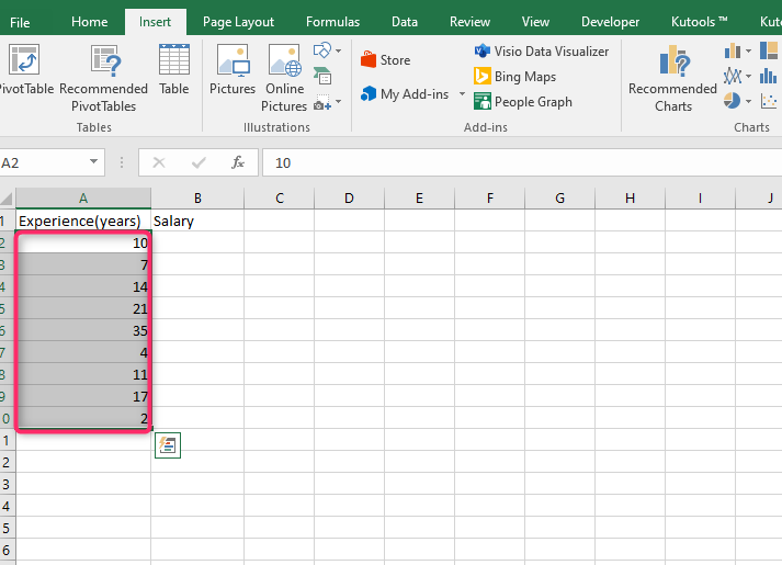
1. To use this function, you need to have the y and x values. Therefore, on the first column of the sheet, enter the data will be used as x values.
2. On the second column, enter the data used as the y values.

3. Select an empty cell and name it to the slope. Then, click on the cell next to the one named slope. This is where you will enter the slope function.

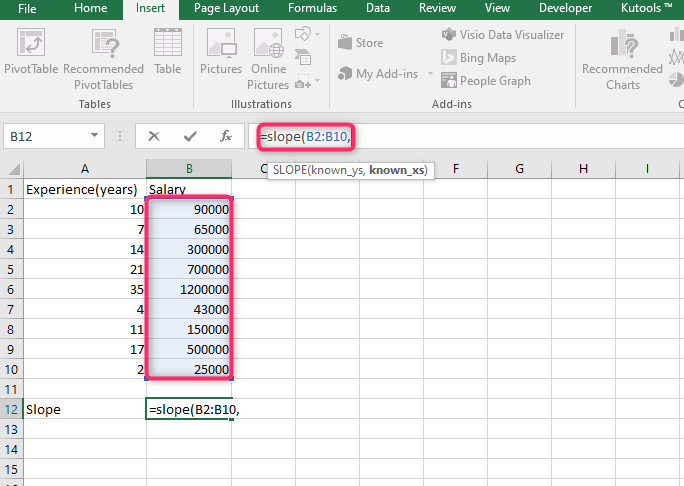
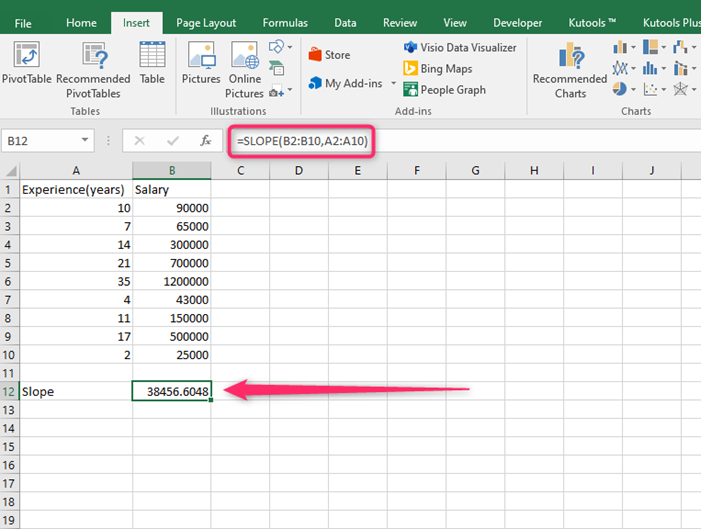
4. Click that cell, and then locate the formula bar. On the formula bar, Enter =Slope(.
5. Then, highlight all the columns that contain your y values. For example =slope(B1:B5,
6. Using a comma, separate the values of y and add values of x. end the function with a closing bracket. For example, =Slope(B1:B5,A1:A5)
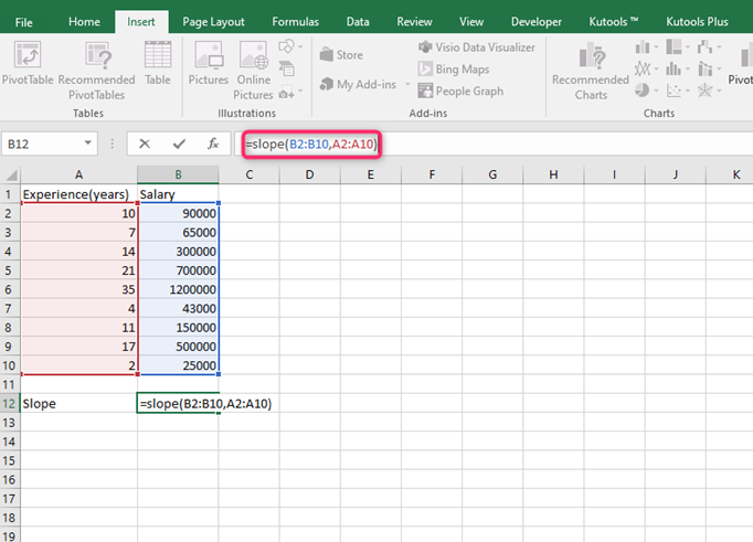
7. Finally, hit the enter button, and the result of the function will be stored on the selected cell.
NOTE:
The Y and X values should be numeric when using this formula.
The values of y should equal the values of x. inequality in values would result in #N/A error.
Finally, this formula can only be used with more than one set of values.
Method 2: Using a chart to find the slope
Another method of calculating the slope of a line is visual charts. This method makes use of the formula Y=mx+c. The m in the formula represents the slope of the line.
To use this method, these steps are followed:
1. On the first column of the sheet, enter; the data will be used as x values.
2. On the second column, enter the data used as the y values.
3. Highlight all the values. That is the X and Y values.

4. Click the Insert tab on the header section. Locate the Insert scatter drop-down menu found in the chart section.

5. Select Scatter. Your values will be converted to a scatter chart.

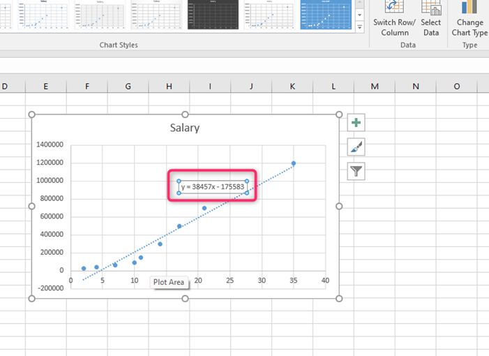
6. Select the chart drawn and click the sign on the top right side. Check the Trendline checkbox.

7. Right-click on the chart and select the Format trendline option.
8. From the Format trendline dialogue box, check the Display Equation on the chart checkbox.
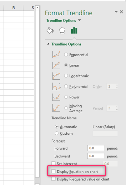
9. Compare the equation displayed with this equation, Y=mx+c.