

When we talk about flipping, we mean turning something upside down. Flipping data in Excel may seem like an inconsequential one-click process, which is not the case as there is no exact in-built Excel feature offering this option. Despite this, you can flip data in excel rows, columns, or tables upside down, vertically or horizontally, using Formula, sort command, or VBA.
Please read the article below to learn different ways of flipping Excel data.
Method 1: Flip data using Sort and Helper columns
It is one of the easiest ways to flip data in excel. You can reverse the order of data, create a helper column beside your primary data and use the Sort command to flip data.
Let's take a look at how to flip data upside down.
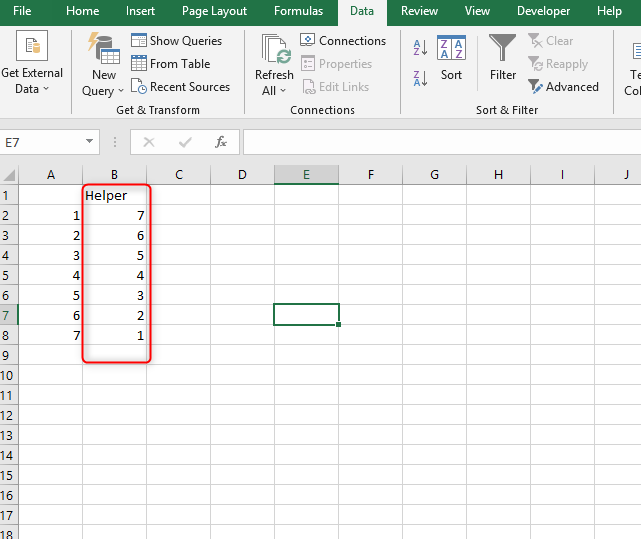
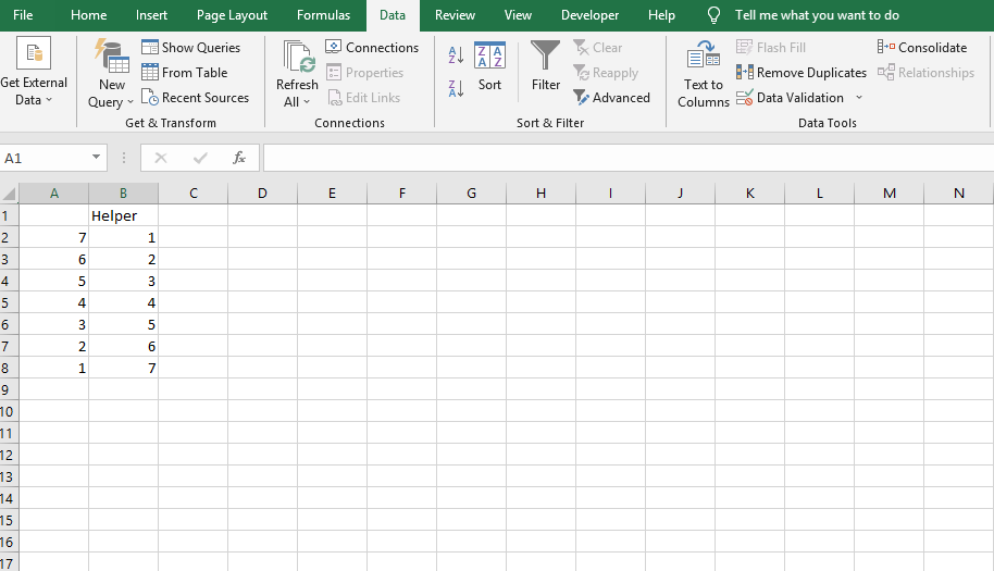
1. In an open worksheet file, create a helper column. You have to make this column adjacent to your main data. Type in the title as Helper.
2. In the helper column, enter a series of numbers going downwards
3. Next, select all your data without forgetting to include the helper column.
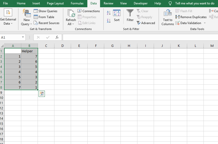
4. Click on the Data tab, which is found in the main menu ribbon.

5. Under the Sort & Filter group, click on the Sort icon to display a dialog box.

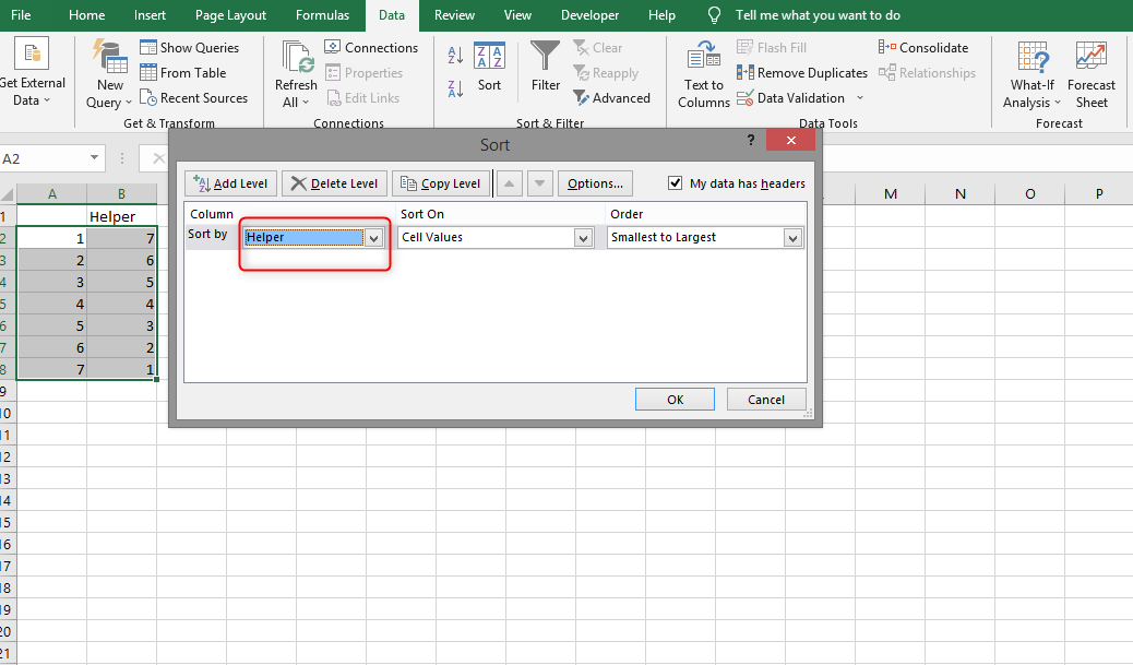
6. In the Sort dialog box, click on the 'Sort by' dropdown arrow. Select the 'Helper' option if you want your results to be based on the helper column. You can pick another preference.
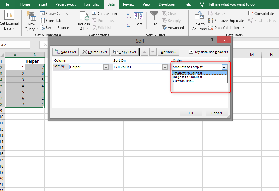
7. Under the Order field dropdown arrow, select Largest to Smallest, Smallest to Largest, or Custom List.
8. On the Sort On field dropdown arrow, select your preference too.
9. Click OK. Your data will be sorted based on your helper column or the option you selected.
In case you want to flip data horizontally, you will still follow the steps above to achieve this. Make sure you first click on the Options tab in the Sort dialog box and check the box 'Sort left to right.'
Method 2: Flip Data using VBA
Using the VBA method to flip data requires a user to create a macro code to run. The beauty of a macro code is that you can either save it in your current book, meaning you can only apply it here. You can also choose to keep it in the Personal Macro Workbook as an add-in to use it in any workbook in Excel. Here is what you have to do;
1. Open the Excel workbook where you want to flip your data.
2. Under the Developer tab, click on the Visual Basic icon to display the Visual Basic Editor window.
3. In the open window, go to the View tab and click on Project Explorer.
4. Right-click any of the objects for the workbook in which you want to add the code. Select the Insert option.
5. Here, click on Module to add a new module to your workbook.
6. In the Project Explorer pane, double-click on the module icon to open a code window.
7. Copy and paste the VBA code below into the code window
Sub FlipVerically()
Dim TopRow As Variant
Dim LastRow As Variant
Dim StartNum As Integer
Dim EndNum As Integer
Application.ScreenUpdating = False
StartNum = 1
EndNum = Selection.Rows.Count
Do While StartNum < EndNum
TopRow = Selection.Rows(StartNum)
LastRow = Selection.Rows(EndNum)
Selection.Rows(EndNum) = TopRow
Selection.Rows(StartNum) = LastRow
StartNum = StartNum + 1
EndNum = EndNum – 1
Loop
Application.ScreenUpdating = True
End Sub
8. Run the macro code. Before doing so, select the dataset you want to flip, go to the VBA editor window and click on the Play button icon in the toolbar to run the code.
Method 3: flipping data in Excel using a formula
You can flip data using a generic formula;
=INDEX (range, Rows (range))
1. In your open worksheet, copy the data headers and paste them where you want the flipped data.
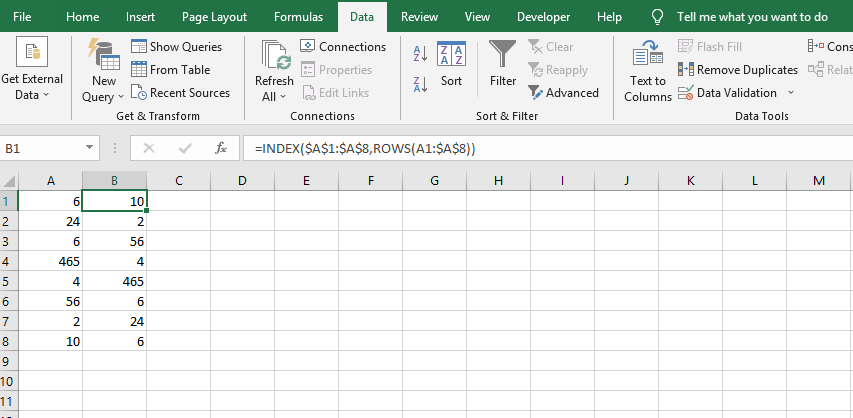
2. Select a blank cell and type in the Formula above. The cell should be in the left-most header.
=INDEX($A$1:$A$8,ROWS(A1:$A$8))
3. Fill in the range of your data and your range rows data.
4. Click Enter when done.
Conclusion
The methods above can be used to flip data vertically, horizontally, or upside down. All you have to do is adjust some of the formulas to indicate how you want your data flipped. I hope you find this article helpful.