

To start it all up, loan amortization is a fancy way to define a loan that is paid back in installments throughout the entire term of the loan. So, all loans are amortized in nature in one way or another. To elaborate all this in a simpler method let me give you an example; if one happens to get an amortized loan for 12months then we will have 12 equal monthly payments, with each payment comes an amount towards principal and some towards interest. To ease up your work, you can create a loan amortization schedule.
An amortization schedule is basically a table that lists periodic payments on a mortgage or loan over time. It breaks down each payment into principal and interest, moreover, it shows the remaining balance after each payment, interesting right? Let's go ahead and identify how to create an amortization schedule.
Method 1: Using inbuilt Excel Template
- Open excel
- Search for Loan Calculator template
- Click create
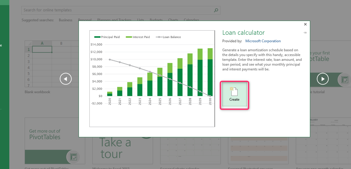
- Fill in the templates with your custom details.
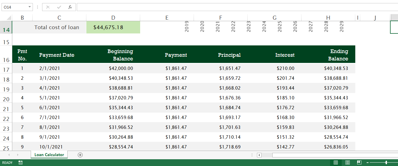
Let us calculate the monthly payment of a loan that has an annual interest of 6%, 2 years of payment, and the amount borrowed to be $42,000. The start date of this loan is 1/1/2021.

- The template will display a summary of the loan repayment. Scroll down to view all the details.
Method 2: Calculate Loan Amortization from scratch
The main requirements that one needs include the following functions:
PMT FUNCTION: This function calculates the total amount of periodic payment. The amount will stay constant for the entire duration of the loan.
PPMT FUNCTION: This function gets the principal part of each payment that goes towards the loan principal, the amount you borrowed. The amount will increase with the subsequent payment.
IPMT FUNCTION: This function finds the interesting part of each payment that goes towards interest. Unlike the above, this decreases with each payment.
Now, let's go through it, step by step:
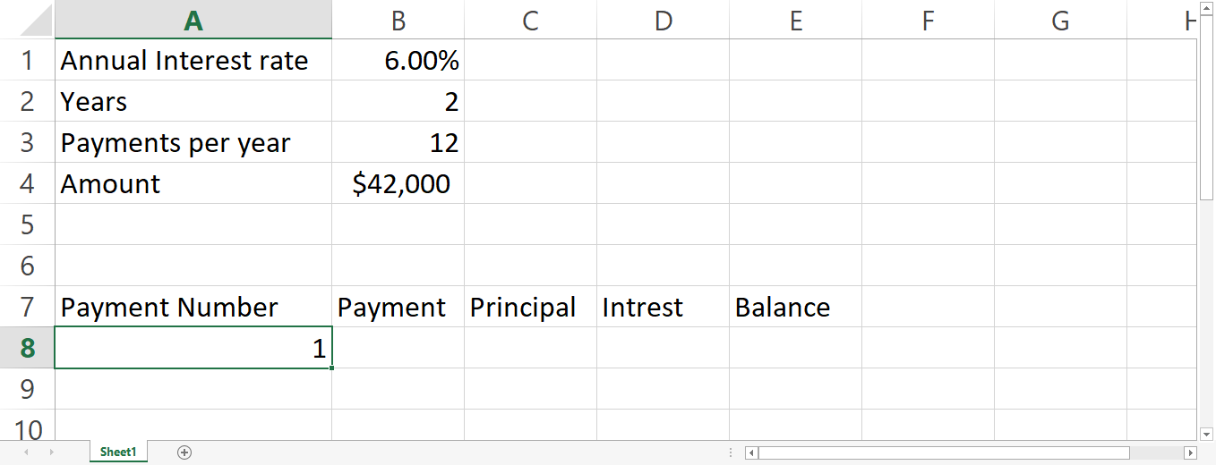
1. Set up the amortization schedule.
Define the input cells where you will enter the known components of a loan which are:
- B1- annual interest rate.
- B2- loan term in years.
- B3 – payments per year.
- B4- loan amount.
After that, we'll create an amortization table with labels (Period, Payment, Interest, Principal, Balance) that should be in A7:AE, in the period column, enter a series of numbers equal to the number of payments, in this case, it's ( 1 – 12).

Let us calculate the monthly payment of a loan that has an annual interest of 6%, 2 years of payment, and the amount borrowed to be $42,000. Let's place our values in the consecutive cells of the template that we have created

2. Use PMT() to calculate the first payment
- For you to get the payment amount, we calculate it with the PMT (rate, nper,pv, [fv] ,[type] function. It is an inbuilt Excel function. First label your first payment on cell A:8
- Now place the cursor to cell B:8 to calculate the first payment. Click on the formula bar at the top left corner and search for the PMT function

The values on the popo up menu represents
Rate: the annual interest rate.
Nper: number of years
Pv: payments per year
FV: The loan amount
Fill in your values to calculate the 1st payment

- Click ok and the first payment will be populated
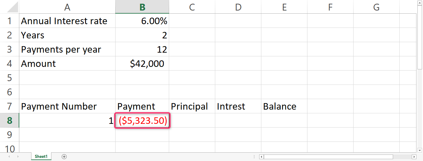
You'll then put the formula together in form of an absolute cell reference, which you'll then copy to the B8 after dragging it down, you'll notice that there's a constant payment amount for all the periods.
3. Find the principal using PPMT ().
- To calculate, the principal part, we'll use the PPMT function. Click on cell C:8 and search for the function.
- Fill in your values in the pop-up menu and press okay

4. Use iPMT() to calculate the 1st interest
Place the cursor on cell D:9 or below the cell that you have labeled interest
- Search for the formula
- Enter your values to the corresponding boxes in the pop-up menu and press okay

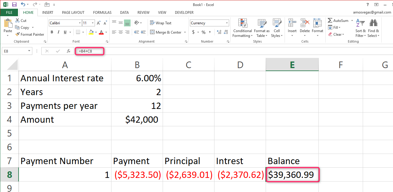
5. Get the remaining balance.
In order to get the remaining balance for each period you can use this formula;
To find the balance after payment the first payment in E8, simply add the loan in B4 and the principal of the first period C8. Thus, B4+D8. Place the cursor on cell E8 and write the formula =B4+D8 on the formula bar and press enter.
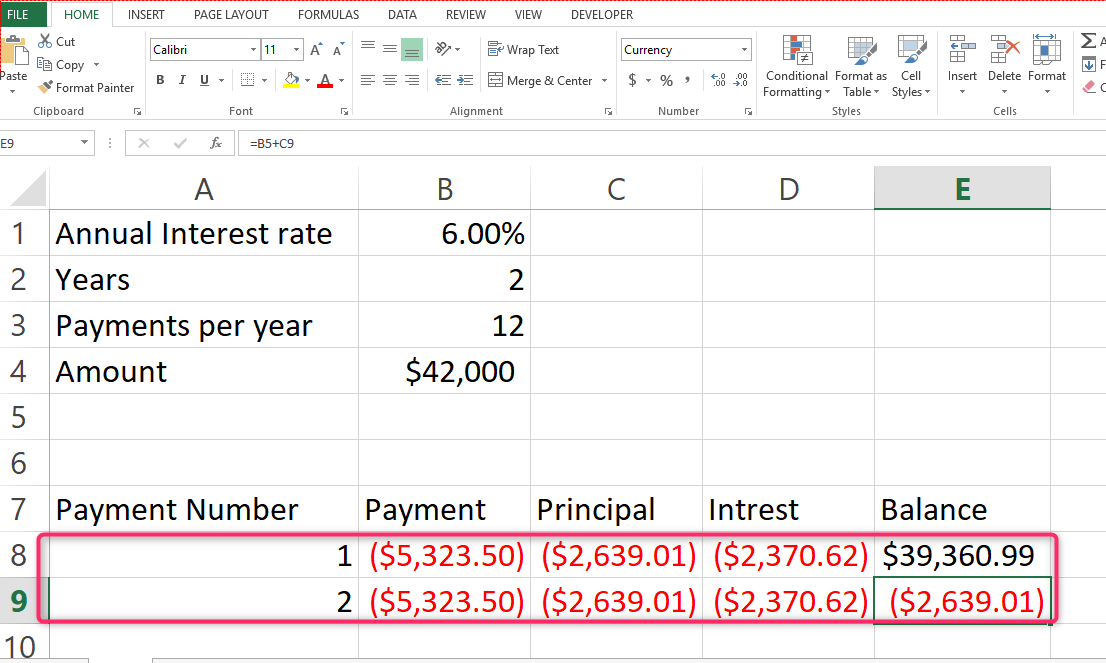
6. Select and drag to the second row
Select range A8:E8 and drag down to the next row
7. Update the balance
Update the balance on E8. Change the formula to E8+c9
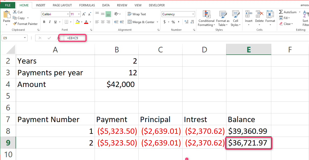
- Update the principal and interest by replacing B4 with E8
- Now select the range A9:E9 and drag up to row 31.