

Microsoft Excel is a good tool when creating reports, forecasts, and budgets. Most companies' excel reports tend to be large hence becoming hard for one to locate certain things. To solve this issue, you can create a search box in excel to look for anything in your spreadsheet. Doing so is very easy and convenient as you will search through rows, columns, or filter data using a specific criterion. The preferable way is using a search box to help an excel user search the entire sheet. Other users may prefer to use the Filter or Find function in Excel though it is limiting as they will need to apply multiple filters to look for different or multiple data.
The article below guides you on how to be able to make your spreadsheet searchable in excel. Let's get started.
Steps to be followed while creating a search box using conditional formatting in excel
1. On your computer, go to the Microsoft Office Suite application and click on Microsoft Excel to open the program.
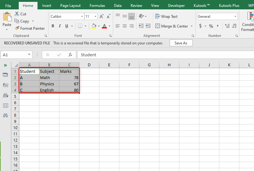
2. In your Microsoft excel program, select the range with the data you need to search by the search box. In our example, we will pick A1:4. But first, we will use cell B1 as our search box. So we will enter a digit equal to cell A4. This will help us to set a conditional format.
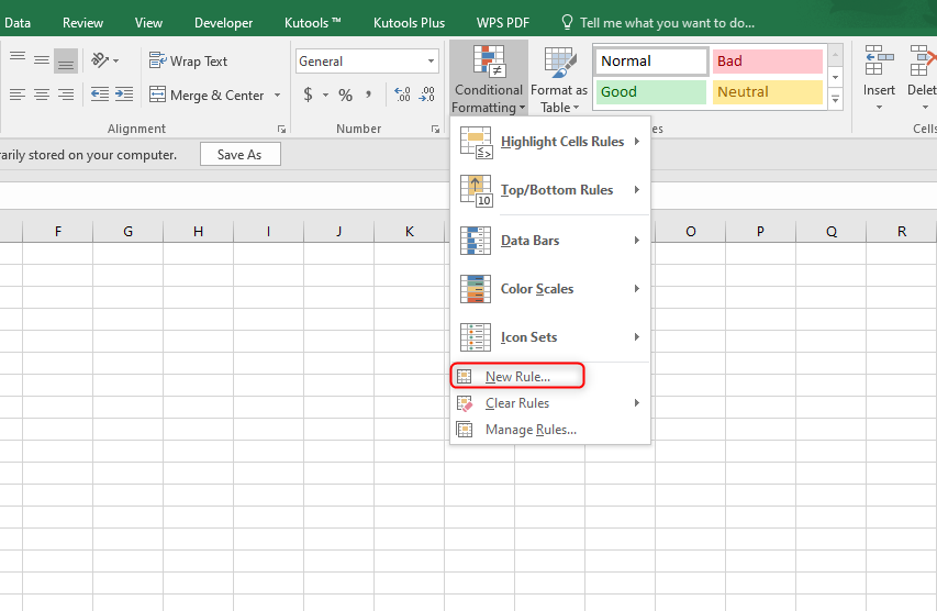
3. On the Home tab under the Styles section, click on the Conditional Formatting drop-down arrow.

4. From the given list, choose New Rule.
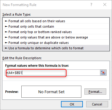
5. In the New Formatting Rule dialogue box, here is what you need to do;
- In the Select a Rule Type box, choose the option 'Use a formula to determine which cells to format.'

- Enter the formula=A4=$B$1 into the box 'Format values where this formula is true.' ( here, fill in the values of where you are searching) where;
=SEARCH is the conditional formatting rule window.
$A$4 defines the location where you apply the search rule. Here you can type in the cell number or click on the blank cell.
A8 specifies the column from which the data is to be searched and the initial position. For example, our formula means that we want to search for column A data, starting from the 8th row.
- Click on the Format button to specify which color you want your searched value to be highlighted. The highlight will be done by selecting the Fill button and selecting the color.
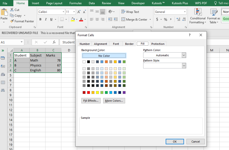
- Click OK. All the selected fields and ranges in your sheet will be highlighted with the selected color.
Note that;
Affixing the dollar sign ($) before cell numbers ensures that the search location will remain fixed even when the search box location is changed. While affixing $ and & at the end means that a user can add more locations from where the data is searched.
Conclusion
The above article gives us a way of making a spreadsheet searchable in Excel. It is the most reliable method when working with large documents in excel. I hope you find it helpful and informative.