
In this tutorial, we will take an in-depth look at some formulas you can use to query a table.
Tables are great in supporting structured referencing; hence, we can use basic formulas to carry out lots of tasks on excel. Without much ado, let's start.

Steps for Querying a table in Excel
We will work on an excel worksheet containing a table – Table 1. The table contains the personal data of the staff of an organization. We can use many formulas to carry out various queries on these data.
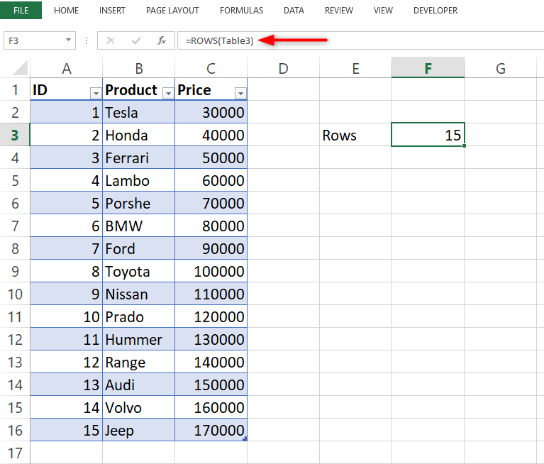
1. Firstly, we will start with the ROWS Function, which we can use to count the rows on the table. It considers only the rows that contain data while counting. There are 15 types of cars on the list.
Here is the formula for the Row function:
=ROWS(Table3)
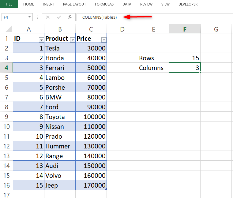
2. We also have the COLUMNS function, which counts the number of columns on the table and considers only the columns containing data.
Below is the formula:
=COLUMNS(Table3)
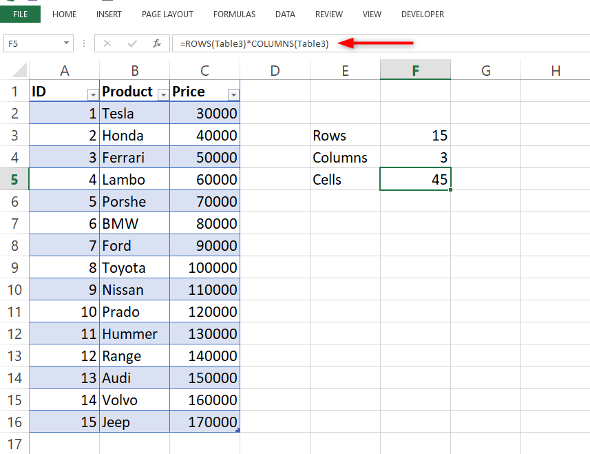
3. Now, if you desire to decipher the total number of cells on the table, you can combine the ROWS and the COLUMNS functions.
Look below for the combo formula.
=ROWS(Table3)*COLUMNS(Table3)
5. Simply use the COUNTBLANK function when you wish to count the cells that contain no data.
=COUNTBLANK(Table1)

6. Another important function is the SUBTOTAL function, which is used in counting visible rows. It is efficient in keeping references to columns that have no empty cells.
The value for ID is a necessity in this case. The ID column represents the reference, and I entered 103 in place of the function number.
=SUBTOTAL(103,Table1[ID])
By entering 103, we tell the SUBTOTAL to only count the values that are invisible rows. The visible row will count upwards when there is no filter but will count downwards if the table is filtered.
Meanwhile, it is important to point out that the SUBTOTAL is very frequent with tables as it has nothing to do with filtered rows.

You can acquire information from the entire row by making use of the #Totals specifier function. Its very simple! Point on it and click.
=Table1[[#Totals],[Group]]
The result of the query will be #REF if you can not see the Totals row.
IFERROR can keep track of the error and return an empty result if you disable the total row.
=IFERROR(Table1[[#Totals],[Group]],"")
If you want to decipher the oldest or newest items on a list, you can use the MIN and MAX functions. The two functions are only potent in a column that contains only numbers.
=MIN(Table1[Start])
=MAX(Table1[Start])
The SUBTOTAL function is the ideal query in case you wish the table to be responsive to filtering. Use it with 105 and 104.
=SUBTOTAL(105,Table1[Start]) — min
=SUBTOTAL(104,Table1[Start]) — max
We also have functions that are efficient in counting groups on tables. COUNTIF and SUMIF functions perform well in this aspect.
=COUNTIF(Table1[Group],I17)
On the whole, all the queries on a table are effective if the range is dynamic. With a dynamic range, your formulas will be updated when you enter more and more data.