
Formulas are key in getting things done in excel. One can apply formulas to manipulate texts, work with dates and time, count and sum with criteria, create dynamic ranges, and dynamically rank values. Explained below are formulas one can apply to remove characters in excel cells.
1. The Array Formula
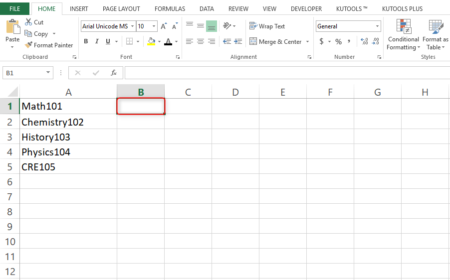
Assuming we want to eliminate numbers from the following data

a) Select a bank cell you will return the text string without the letters.
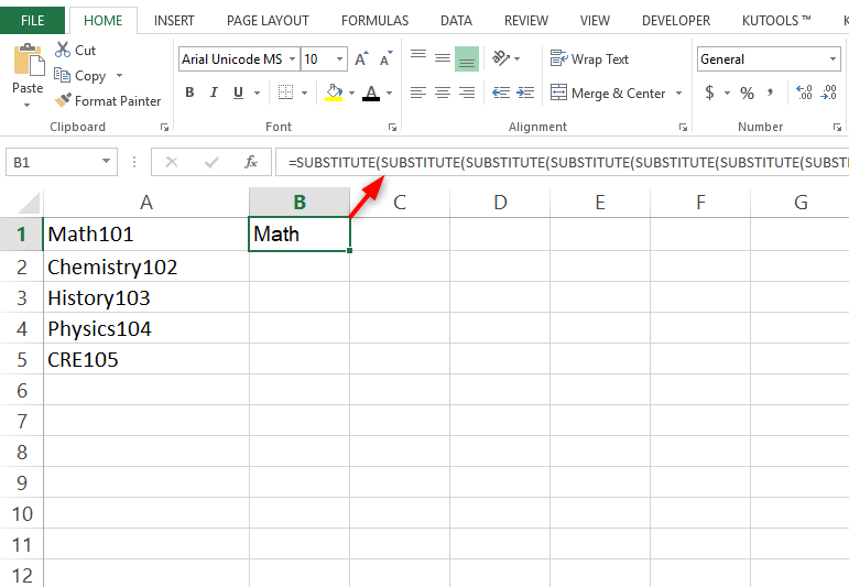
Enter the formula;
=SUBSTITUTE(SUBSTITUTE(SUBSTITUTE(SUBSTITUTE(SUBSTITUTE(SUBSTITUTE(SUBSTITUTE(SUBSTITUTE(SUBSTITUTE(SUBSTITUTE(A1,1,""),2,""),3,""),4,""),5,""),6,""),7,""),8,""),9,""),0,"")
(A1 is the cell you will remove characters from) into it, and press the Ctrl + shift + ENTER keys all at the same time.
b) Keep selecting the cell and then drag its fill handle to the range as you wish. You will now see all letters removed from the original text strings.
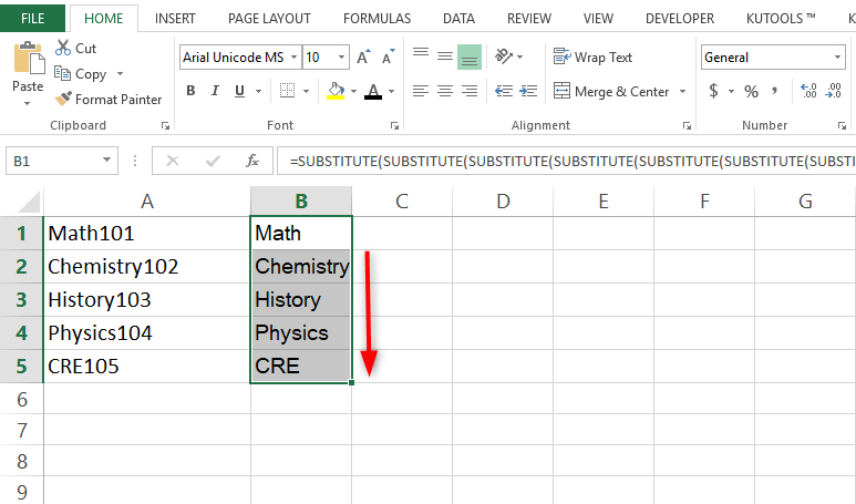
N/B: This formula removes all kinds of characters except numeric characters. If there's no number in the text string, this array formula will return zero.
2. User of Defined Functions
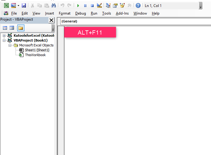
a) Press Alt + F11 keys simultaneously to open the Microsoft Visual for the app window.
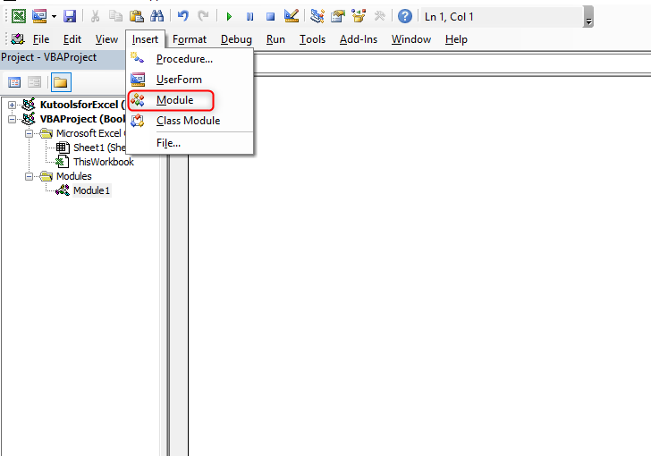
b) Click insert> module and then copy and paste the following code:
Function RemoveNumbers(Txt As String) As String
With CreateObject("VBScript.RegExp")
.Global = True
.Pattern = "[0-9]"
RemoveNumbers = .Replace(Txt, "")
End With
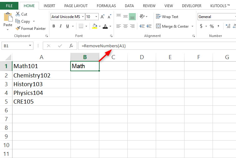
End Function Code source:Extendoffice.comc) The user-defined function is then saved. A blank cell is selected where a text without strings is returned. Later, the Fill handle s dragged down to the ranges after entering the =removenumbers(A1)
N/B: This function can also remove all kinds of characters except numeric characters and return numbers stored as text strings.
3. Excel Left Function
(EXCEL LEFT) the function enables left side extraction of characters in a given text. For instance, LEFT ("apple", 3) returns "app" In our example above we will use =left(A1,4)
4. Kutools for Excel

All characters can be removed by the methods mentioned above
The Kool method is applied where one only needs to remove letters from the text and remain with numeric characters. This method will introduce Kutools is essential in removing characters utility in Excel
For it's for easiness.
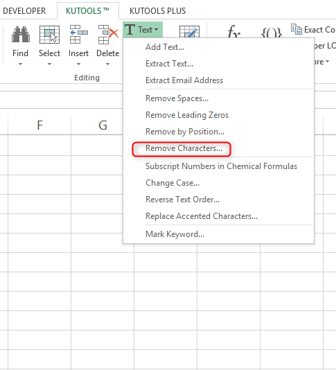
a) Select the cells you will remove letters from, then click Kutools>text> Remove characters.
b) In the opening remove characters dialog box, check the Alpha option and then click the OK button.
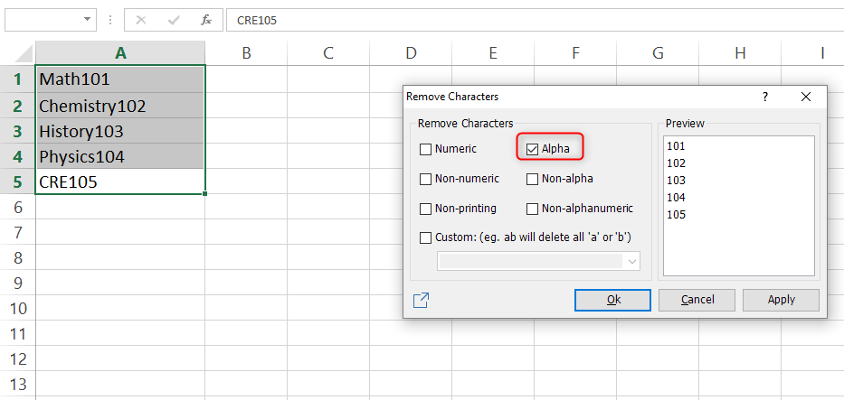
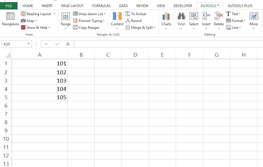
You'll see only letters are removed from select cells.
N/B: If you want to remove all kinds of characters except the numeric ones, you can check the non-numeric option and click the OK button in the remove character dialog box.
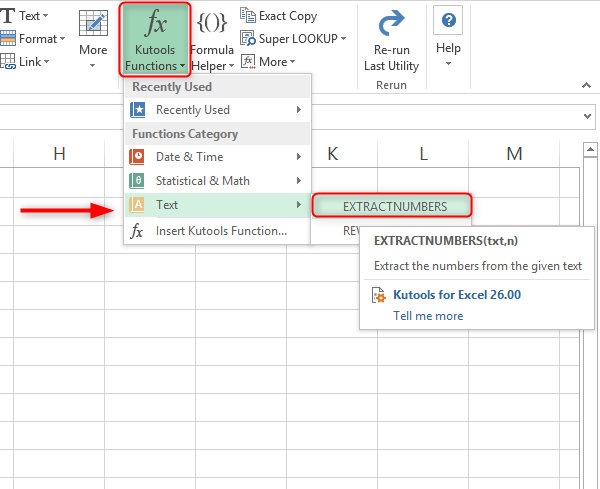
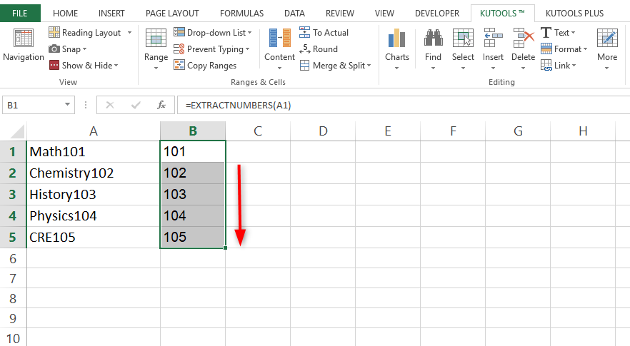
5) Extract Numbers Function of Kutools For Excel.
a) Select a blank cell, you will return the text string without letters and click Kutools>functions> texts> text> EXTRACTNUMBERS.
b) Specify the cells to which letters should be removed and replaced in the TEXT box. The specification should be done in the opening dialog box. The TRUE or FALSE is not compulsory. I typed into the N box and clicked the OK button.
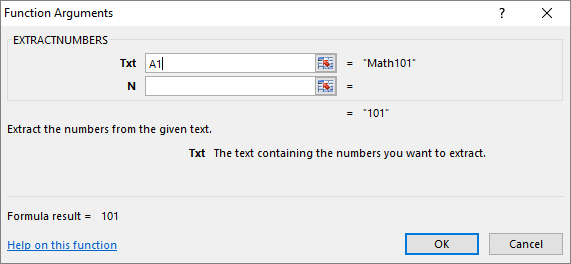
c) Keep selecting the cell and drag the fill handle to the range you need. You'll see all letters removed from the original text strings.
5. Using Find and Replace Feature to Remove Specific Characters
The Find & Replace feature allows you to remove unnecessary characters to give the desired result. For example, if you have a dataset full of irrelevant dots, you can remove the dots and get a clean and organized dataset by following these steps:
a). Select the dataset you want to clean or remove irrelevant characters.
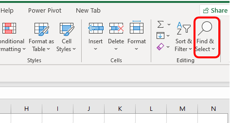
b). Go to the Home ribbon and click on Find & Select.
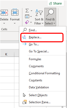
c). From the drop-down menu, select the Replace option.
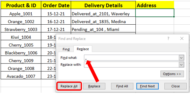
d). A new Find and Replace pop-up box will appear. Go to the Find with field and write dash (_).
e). Leave the Replace with field blank.
f). Click the Replace All button and you will delete all unwanted dots from your dataset.
6. Removing Specific Characters with The SUBSTITUTE Function
Since using an Excel formula is the most controlled way to remove characters, you can use the SUBSTITUTE function to get the desired result without any specific character. The generic formula of the function is;
=SUBSTITUTE(cell, “old_text”, “new_text”), where;
old_text is the text or characters you want to remove.
new_text is the text or characters you want to replace with.
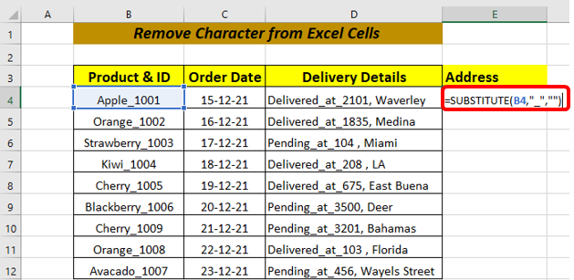
Using the same dataset with messed dots as above, you can remove the dots with the SUBSTITUTE following these steps:
a). Start by writing the equal sign (=) followed by SUBSTITUTE in the cell where you want to result to appear.
b). Open the brackets and write the cell reference number from which you want to remove the character. For example, you can write C5 if the messed data is in cell C5.
c). Put a comma (,) and write dot (.) or any old text you want to remove inside double quotes.
d). Put another comma (,) and leave a blank double quote. You can also write your desired new text inside the double quotes and close the bracket. Your final formula will look like this:
=SUBSTITUTE(B4,”_”,””)
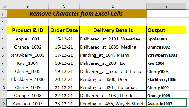
e). Press the Enter button. You will see all the dots or unwanted characters removed from your data.
f). You can now use the Fill Handle to drag the formula down the column to fill the rest of the cells.
7. Removing A Specific Character from A Particular Position
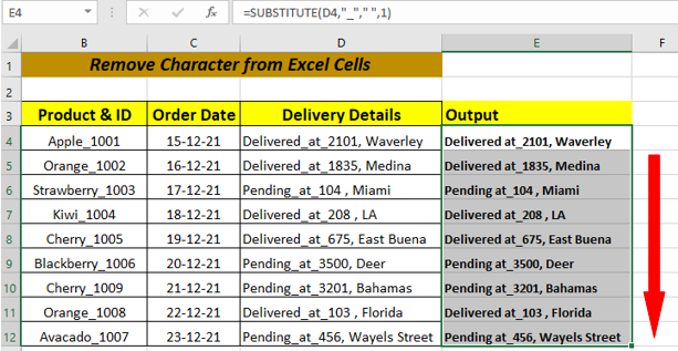
Unlike the above procedure that removes dashes (_) from positions, this method allows you to remove specific characters from a particular position. The generic formula will remain almost the same, but with a number at the end that defines the position of the unwanted character. Therefore, if you want to remove the first character from a text in cell D4, the formula will become:
=SUBSTITUTE(D4,”_”,” ”,1)
If you want to remove a character from any position, you only need to replace 1 with the position of the character, such as 2, 3, and so on.
Steps
a). Write the formula in the cell next to the dataset you want to modify. For example, if the data is in cell D5, you can write the formula in cell E6.

b). Press the Enter button and you will see a new text without the character.
c). You can now use the Fill Handle to drag the formula down the column to generate results for the rest of the cells.
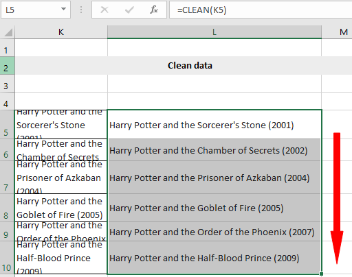
8. Using The CLEAN Function to Erase a Specific Character
The CLEAN function is essential if you have copied a large dataset with unnecessary characters such as new-line, dots, spaces, and many more. It can also remove line breaks and non-printable characters from a string in Excel. Its syntax is;
=CLEAN(original_string), where;
original_string is the cell reference of the text you want to clean.
Steps
a). Select the cell where you want to store the result. You can select C5 if the messed data is in cell B5.
b). Write the following formula in the selected cell.
=CLEAN(K5)
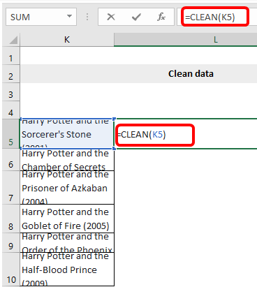
c). Press Enter and you will see clean data without line breaks or unnecessary data.
d). Use the Fill Handle to drag the formula down the column.
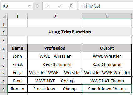
9. Using The TRIM Function to Remove Space Characters
The only downside with the CLEAN function is that it removes only the first 32 (non-printable) characters in the 7-bit ASCII code. That means it cannot remove the space character since the space character has a value of 32. Therefore, to remove the space character, you may need to use the TRIM function which removes all extra space characters and gives a dataset with only a single space. Its syntax is:
=TRIM(original_string), where;
original_string is the cell reference of the text you want to trim.
Steps
a). Select the cell where you want the new text to appear. For example, you can pick cell D5 if the messed data is in cell C5.
b). Write the following formula in cell K5.
=TRIM(J5)
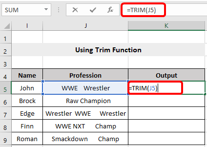
c). Press the Enter button. This will give a new text with all unwanted spaces removed.
d). Use the Fill Handle to drag the formula down the rest of the cells.