Reminders or notifications can be inserted into the excel document for purposes. This date reminder plays a vital role in ensuring a certain activity is not omitted and is done at the right time. Many users do not know this excel feature, and therefore only a few may realize the benefits behind it. However, others may have heard of it but using it becomes a challenge. This article makes it easier for any user who wants to use the reminder feature of Excel.
We shall discuss two methods that you can comfortably use to set a reminder:
- Use the IF function to display a message
- Use conditional formatting
Use the IF function to display a message.
In this method, the IF function is used to display a reminder message if the date is due to the set date. The following steps should be followed if this method is used:
1. Open your excel document where you want to set the date reminder or the notification.
2. If the document is empty, you can add the data on the cell alongside dates.
3. Separately, from the column that contains the information and the date, create a new column called Remarks. This is the column that will contain the IF function reminder.
4. Write an IF function next to the date on each row that contains the data.
Formula: =IF(B2<TODAY()+2,”send reminder”,””)
Below is an example:
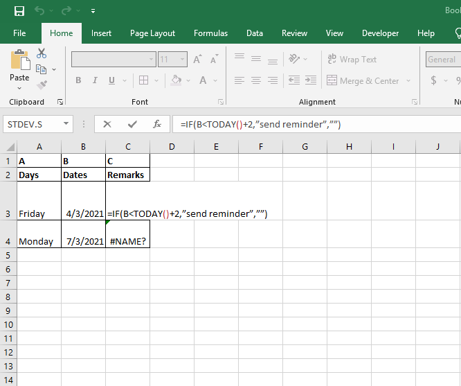
The above table shows how the If the function can be inserted into the excel cells. According to the above example, B refers to the column where the date is located, +2 is used to remind the user two days earlier, and the phrase "send reminder" is displayed when the reminder date has reached.
Use of conditional formatting
In this method, the following steps are encountered:
1. Fill the excel file with the required data, i.e., the date and the date information.
2. Then, highlight the dates in the date column.
3. Go to the "Home" tab on the excel page. This is found on the uppermost part of the screen. Click on this button.

4. Locate and click the "conditional Formatting" button, creating a new formula.

5. Once you've clicked the conditional formatting button, a new page with the title "New Formatting Rule" opens. It is on this page that you will add the AND formula. The AND formula is responsible for comparing two conditions. An example of the AND formulae would be:
=AND (B<> "", B<TODAY () +2)

6. Formatting involves formatting and customizing how the reminder will look if the conditions are met. The operation involved in this step includes: editing the border color, the font style, the fill inside, and the font color.
7. Then click "OK" to complete the customization and the process of setting a reminder. If the date is two days due to the set date, the date will be highlighted.
Combining TODAY, AND, and IF Functions
Combining TODAY, AND, and IF functions can sound like a complicated way to set date reminders in Excel. However, it is the easiest way to set reminders for several days ahead. For instance, combining all the functions allows you to check seven days ahead of the current date.
When setting reminders, the formula will return YES if any date passes the due date and NO if no date passes the due date. Therefore, you need to create another column to store the return text.
Steps:
1. After creating another column, say cell E5, type in the following formula:
=IF(AND(D5<>"“, TODAY () +$D$11>=D5),"Yes","No"), where;

TODAY () +$D$11>=D5 checks the range of seven days ahead of the current. It should TRUE whether the range is greater or equal to the date in cell D5.
D5<>”” checks if cell D5 is empty or not. It should also return TRUE.
AND(D5<>””, TODAY () +$D$11>=D5) – The AND function combines both outputs and returns FALSE if any output goes FALSE. It will also return TRUE if both outputs are TRUE.
Therefore, the IF function in the formula will return YES for TRUE output and NO for FALSE output.
2. After writing the formula, press the Enter button, and the formula will show up in the formula cell.
3. Use the Fill Handle icon to drag and copy the formula in other cells.

4. Finally, you will have your outputs in each corresponding cell.
Embedding VBA Macro to Get Pop-Up Alerts for Due Dates
The method is ideal for people who love working with codes since it allows them to set date reminders easily. It also gives pop-up notifications with other vital details such as daily schedules and names. To use the VBA Macro code to set reminders, follow these steps:
1. Right-click on the sheet title.
2. Select View Code from the Context Menu.

3. The VBA will open and show the following code:
Option Explicit
Sub Due_Date()
Dim DueDate_Col As Range
Dim Due As Range
Dim PopUp_Notification As String
Set DueDate_Col = Range("D5:D9")
For Each Due In DueDate_Col
    If Due <> "" And Date >= Due - Range("D11") Then
        PopUp_Notification = PopUp_Notification & " " & Due.Offset(0, -2)
    End If
Next Due
If PopUp_Notification = "" Then
    MsgBox "No need to chase any buyer today."
Else: MsgBox "These buyers need chasing today: " & PopUp_Notification
End If
End Sub
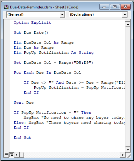
4. Copy and paste the codes into the cell.
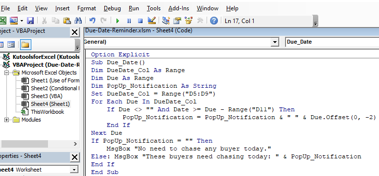
5. Press the Run icon to run the codes and you will have a pop-up notification on every due date.
Using Kutools for Excel to Select and Highlight the Approaching Due Date
If you already have Kutools for Excels installed, you can use its Select Specific Cells utility to select and highlight the approaching due dates quickly. However, if you don’t have Kutools for Excel, you will need to install it to apply its utilities in setting date reminders. After installing, you can proceed with the following steps:
1. Select a blank cell next to the dates you want to set reminders for. For example, you can select cell E5 if the due date is in cell D5.

2. Type the formula below in the cell, which gives a date that is N days from the current date.
=TODAY()+N, where;
N represents the number of days you want the alert from the current date.
3. Select the dates you want to highlight approaching dates.
4. Now click on Kutools tabs > Select > Select Specific Cells.
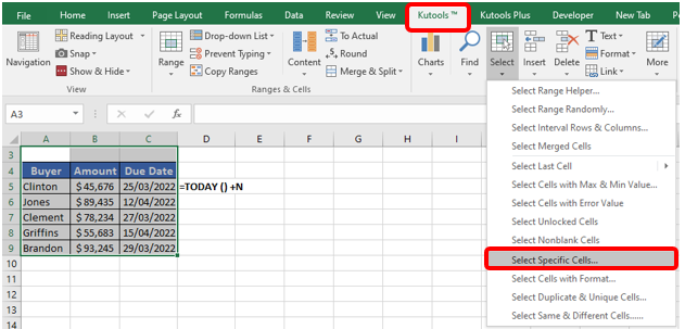
5. When the Select Specific Cells dialog box opens, go to the Specific Type section and select the Less Than option from the drop-down list.
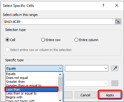
6. Next, click on the arrow box on the right end to select the formula cell you used in the first step above.

7. Click OK, and you will see the approaching dates selected. You can highlight them with any background format of your choice.
