

I am sure you must be wondering, "what is VLOOKUP and what exactly does it do in Excel?" Well, it turns out it is among the most popular functions in Excel. VLOOKUP is an Excel database function that mostly deals with lists in Excel or any database table. It is a useful function though also overlooked by most Excel users as they perceive it to be hard to understand what it does. Its primary function is to look up and retrieve data from a specific column in a table and match it on the first column. For the VLOOKUP function to work with a given list, the list must have a column containing a unique identifier or ID. The ID also has to be the first column in your data table.
The VLOOKUP function is a syntax that contains four pieces of information that you will need. It is,
=VLOOKUP (lookup_value, table_array, column_index, [range_lookup]) where,
1. Lookup_value– it is the value to look up in the first column of a table.
2. Table_array– where you want to look for it
3. The column_index-the column number in the range containing the value to return or retrieve
4. Range_lookup-return an approximate match= (optional) TRUE or Exact match = FALSE. If you don't specify anything, the default value will be an approximate match.
Let's look at how to use Excel VLOOKUP.
Steps to be followed when using VLOOKUP wizard
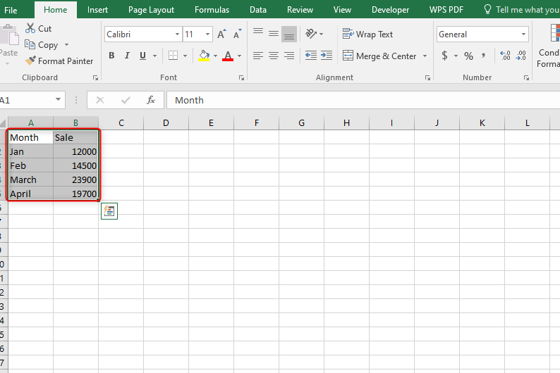
1. Open an Excel worksheet that contains your data.
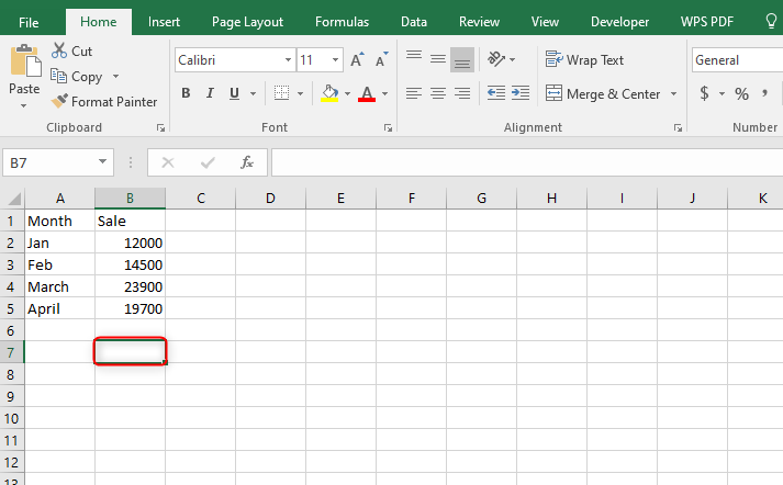
2. Locate where you want the data to go and click that cell only once. You can choose any cell below or beside your data.
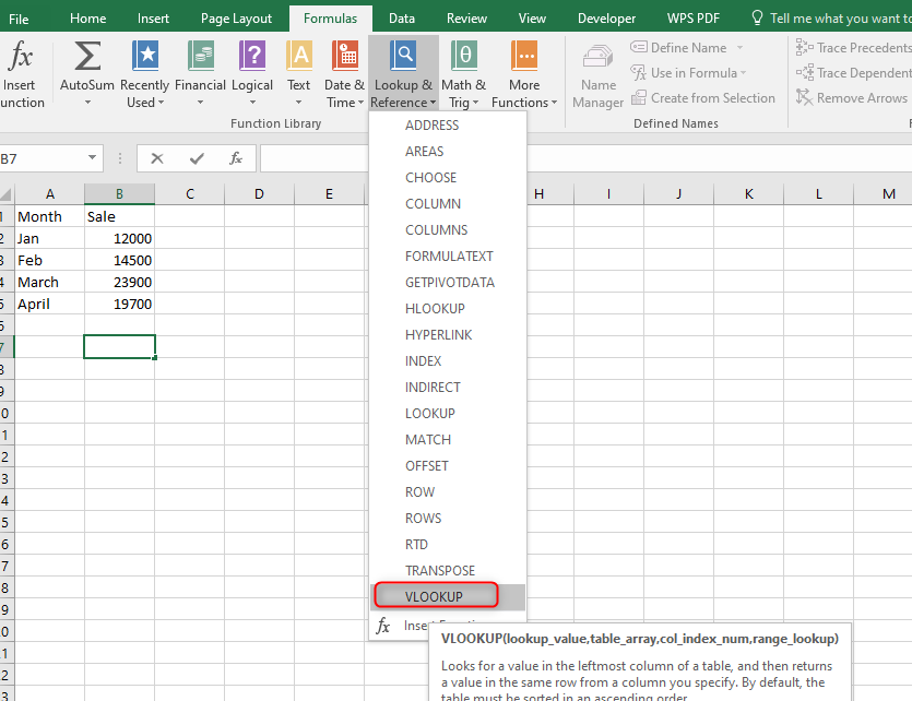
3. At the top of the main ribbon menu, click on the Formulas tab.

4. Under the 'Function Library,' go to Lookup & Reference. Click on the drop-down arrow.

5. From the given options, select VLOOKUP.
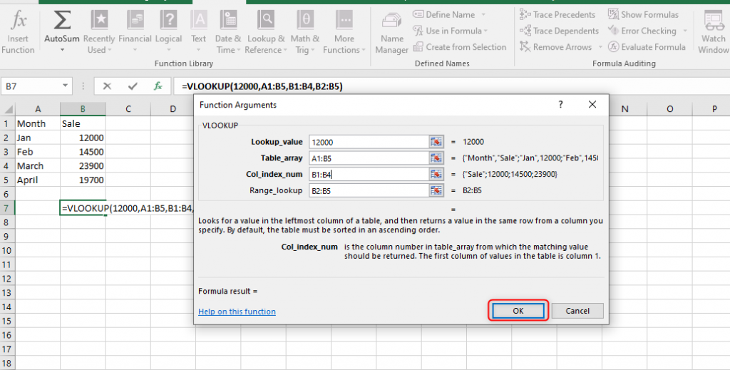
6. Excel's VLOOKUP pop-up wizard will be displayed. The window contains all the parts of the formula.
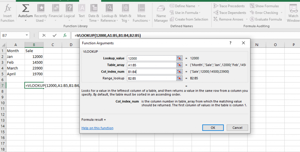
7. Click OK when you are done.
Note that you can manually type in your formula in the empty cell you selected in cases where you don't want to go all the way to the VLOOKUP wizard window.
VLOOKUP Parameters
- Lookup_value. Find the unique identifier from your data. The ID is usually in the same row as the empty cell you selected in step 2. Click on it for that cell to be filled.
- The next field we are looking at is, Table_array. Go to your table and highlight the information you want. Start by highlighting the unique identifier. To avoid confusion and inaccurate data being selected, ensure that all your unique IDs are listed only once in the table_array field.
- In the Column_index, look for the column that contains the information you want to be retrieved. You will type in the number of columns your field is from the unique ID. For example, if your value is in the fourth column after the unique identifier, write 4 in the Column_index field.
- Lastly, go to Range_lookup. Here type FALSE, and Excel will search for the exact matches. You can also type TRUE to view your data as an approximate match.
Conclusion
I hope you can access and use the VLOOKUP function with the article above while working with Excel worksheets. The steps are easy enough to follow.