
VLOOKUP is one of the most useful Excel functions. The function is used to search for specific values defined and returns the match-in value from another column. The VLOOKUP function, just as the name looks up a value in the first column of a specified range of cells and then returns the results on the same row from another column.
The "V" in VLOOKUP stands for vertical, thus data in the table is vertically arranged with data in the rows. When information is arranged vertically with columns on the left, data can easily be retrieved by matching rows with columns on the left. V differentiates VLOOKUP from the HLOOKUP which looks for values on the top row of an array horizontally.
Syntax:
VLOOKUP(LOOKUP_VALUE, TABLE-ARRAY, COL_IDEX_NUM, [RANGE_lOOKUP])
VLOOKUP Parameters:
The VLOOKUP function has four parameters or arguments. The first three parameters are a requirement whereas the last parameter is optional.
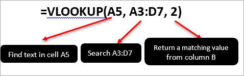
1. Lookup_value: the value you're looking for and it can be a number, date, text, or a cell reference.
2. Table_array: It is the range of cells that make up the table or array of data to be searched. The function searches a value in the first column of the table_array.
3. Column_index_num: It is an integer specifying the column number from which to retrieve a result.
The left column in the table_array is 1, the second column is 2, and so on.
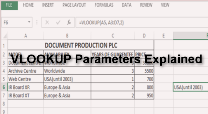
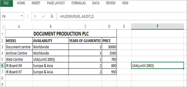
In the example below we will look for "web Centre" in cell A5 and return the matching values from column 2 for the specified table_array A3:D7.
1. [Range_lookup]: The match mode. It describes what function should be returned in the event an exact match is not found in the lookup_value.
The range_lookup can either be true or false.
TRUE means approximate or closest match below the lookup_value
FALSE means exact match to the lookup_value is not found and returns an error.
| Name | Installment 1 | Course | Installment 2 |
| Jennifer | 7000 | Accounts | 2000 |
| Jane rose | 7500 | Secretarial comps | 500 |
| Victor | 6000 | Pharmacy | 2600 |
| Ambrose | 6100 | Accounts &Comps | 1200 |
| Kennedy | 7000 | Pharmacy | 2000 |
| Melvin | 10000 | Pharmacy | 2200 |
| Christian | 6000 | Secretarial | 1300 |
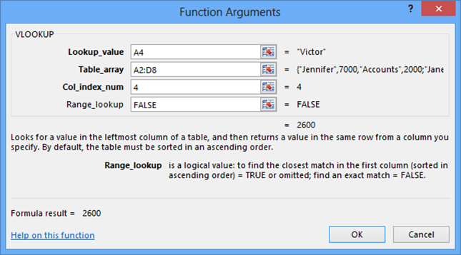
In the above example to get the matching value of 2nd installment for the victor, put your cursor in a blank cell at a column on the right and insert the Vlookup function.
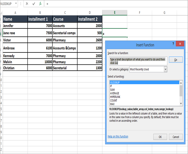
Select VLOOKUP and click OK to open the VLOOKUP Windows
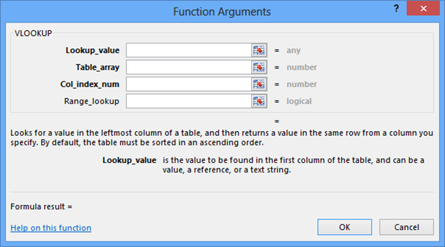
Enter the VLOOKUP parameters or Arguments
Click OK
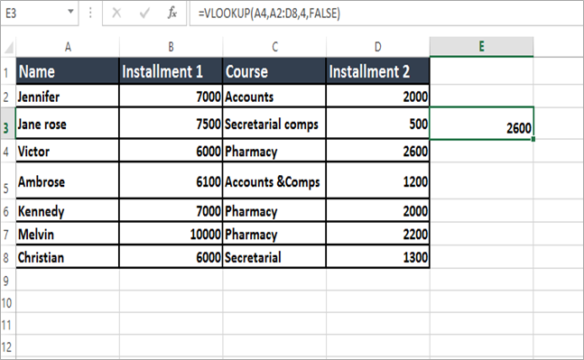
NOTE: Vlookup function searches in the left-most column of an array.